If you have a homogeneous multi-machine Linux/GCC environment such as a Beowulf cluster and are performing long-running analyses, you may be able to benefit from using compiled polynomials, which can provide an order of magnitude improvement in evaluation performance, and a degree of reusability.
In order to understand the value of polynomial compilation, one must first understand what polynomials are and how Kelvin uses them.
When Kelvin performs an analysis, the majority of the work is calculating the likelihood of every pedigree's structure and characteristics for each combination of values in the trait model space, which is typically a range of 6 gene frequencies, 275 penetrances, and 20 alpha values, or 33,000 combinations of values. This is repeated for each trait position in the analysis.
In (original) non-polynomial mode, the pedigree likelihood is explicitly calculated via a series of tests, loops and arithmetic operations in the compiled code that comprises Kelvin. Since these tests, loops and operations are all hard-coded in the program, they cannot be optimized or simplified in response to the nature of each pedigree, so the same full series of steps is followed for every combination of values.
In polynomial mode, we go thru this same hard-coded path in Kelvin one time only building a symbolic representation of the calculation using place-holder variables from the trait model space instead of actual numeric values. In effect, we build a polynomial that represents the structure and characteristics of the pedigree in terms of the variables from the trait model space. This polynomial representation can then be extensively simplified and optimized using mathematical and computational techniques so that when we assign trait model space values to the place-holder variables and evaluate it, it can perform the calculation orders of magnitude faster than the original hard-coded path in Kelvin.
This process of generating polynomials has its own drawbacks. They can take a lot of time and memory to generate and optimize, and even when optimization is complete, their evaluation is symbolic and therefore slower than the equivalent binary operations. Ideally, we'd like to have both the optimized simplicity of the pedigree/position-specific polynomial and the performance and reusability of compiled code. The solution is to generate and compile code representing each polynomial.
During a polynomial-mode analysis, a separate set of likelihood polynomials is built for each pedigree and combination of relative trait/marker positions. For example, a multipoint analysis with two pedigrees and three markers where evaluated trait positions occur between every pair of markers as well as before and after the markers would generate twelve polynomials:
The trait and marker likelihood polynomials are extremely simple compared to the combined likelihood polynomials. Marker likelihood polynomials usually simplify to a constant, while combined likelihood polynomials usually have tens of thousands, and sometimes even billions of terms.
Polynomial compilation is a method of post-processing a discrete, nameable, in-memory polynomial generated by Kelvin so as to facilitate rapid evaluation and reuse. By discrete and nameable, we mean that all information required for the construction of the polynomial is available before construction begins, and that there are a relatively small number of attributes that can be used to distinguish this particular polynomial from other similar ones and therefore comprise a unique name. Fortunately, Kelvin has been written in such a way that all major polynomials generated are both discrete and nameable.
When polynomial compilation is used, likelihood polynomials are built in-memory as usual in an initial Kelvin run, and then translated into C-language code and written to one or more source files which are then compiled into dynamic libraries. These dynamic libraries are reusable, distributable, compiled representations of the original polynomials that can be loaded on-demand and evaluated up to ten times faster than their original in-memory counterparts.
Once a dynamic library is built for a given polynomial, the relatively slow and memory-intensive process of generating that polynomial need not be performed again unless one of the following changes:
While compiled polynomial names incorporate enough information to uniquely identify them within a given analysis run, they do not contain an exhaustive description of the analysis, so it is important to be careful to remove any existing compiled polynomials (*.so files) when one of the aforementioned characteristics changes, otherwise Kelvin might crash, or worse -- the analysis results will be incorrect. You can, however, freely change any of the following analysis characteristics and still take advantage of any pre-existing compiled polynomials:
Generally, you should use polynomial compilation only when it is technically feasible in your computational environment and the cost and complexity of compiling and linking dynamic libraries is exceeded by the benefits of rapid and repeatable evaluation.
Compiled polynomial use consists of several phases that have very different requirements and optimization possibilities:
Polynomial build and code generation. This is pretty much the same as the normal process of polynomial building that occurs whenever you use the PE directive in your analysis, coupled with the fairly quick additional step of generating a number of C-code files to represent the polynomial. This step is only performed if there is not already a compiled polynomial of the same name in the current default directory. As with the normal polynomial build process, this step can be very memory-intensive depending upon the structure of the pedigrees and number of positions in the analysis, and does not benefit significantly from running in a multi-threaded environment.
Code compilation and dynamic library (DL) linking. Compilation can be performed at the time the source is generated by Kelvin itself, or by way of batch jobs submitted on multiple nodes. Both approaches require:
polynomial.h and polyDLLoop.c from the distribution pedlib/ directory copied to somewhere on the GCC include file search list, i.e. in /usr/local/include or in a directory specified by the CPATH environment variable.compileDL.sh from the top-level distribution directory copied to somewhere on the command path, i.e. in a directory specified in the PATH environment variable. This script file is executed from within Kelvin to build dynamic libraries, and should be protected from unauthorized modification, as it would otherwise present a potential security risk. Currently this script moves source files to a compiled subdirectory once a dynamic library is built. You may wish to modify it's behavior or change the compilation optimization level.This step is only performed if code has been written and synchronous compilation specified.
The source files generated are currently sized to be as large as can be compiled in under 16Gb of physical memory in order to facilitate optimization, and are compiled serially, so this step does not benefit at all from running in a multi-threaded environment.
Compiled polynomial loading and evaluation. An attempt is made to locate and load a dynamic library (.so file) for each polynomial (one per pedigree) required for evaluation at a specific position before evaluation begins. Only the current execution directory is searched -- not the normal default dynamic library paths, as moving the dynamic libraries out of their associated analysis directory would facilitate accidental misuse. Any polynomials not represented by an existing dynamic library are built, and may be coded, compiled and loaded. Evaluation of the polynomials for a position is done in parallel by pedigrees, and so takes advantage of a multi-threaded environment insofar as the pedigrees are of similar complexity.
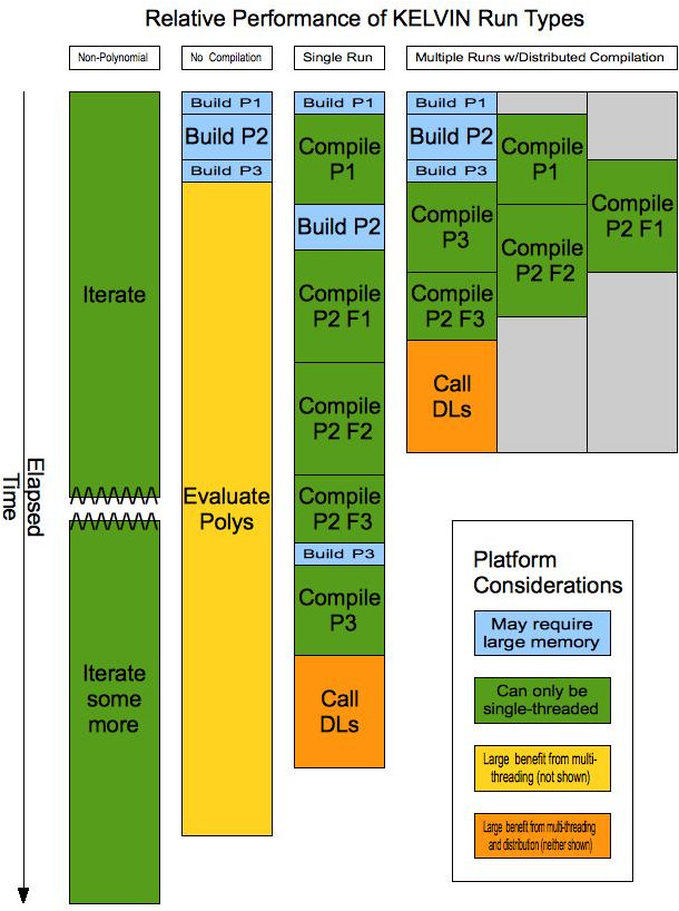
As the different phases of compiled polynomial processing have very different performance characteristics, two distinct mechanisms have been setup in Kelvin to support them. The first is a simplistic linear single-run approach which does not fully exploit performance capabilities, but can provide a significant performance boost over regular polynomial processing. The second is a relatively complicated multiple run process that achieves maximal performance. This chart illustrates the performance characteristics of these two approaches, along with the characteristics of a non-polynomial run and a polynomial run without compilation. The illustration assumes a simplified case where there is a single trait position for which three significant polynomials are generated (P1, P2, and P3), two of which are simple enough to be described by a single source file (P1 and P3), and one which requires three source files (P2 F1, F2, and F3).
The Kelvin binaries referenced below can be produced by executing make specialty in the top-level distribution directory. A future release of Kelvin will combine them all into a single binary whose operation will be controlled by command-line options.
kelvin-normal binary without the PE directive in the configuration file. It requires very little physical memory, but has a relatively long execution time which cannot be improved with multi-threading. Total run-time is easily and accurately extrapolated from initial progress, so a decision can be made fairly quickly as to whether this approach is worth pursuing.kelvin-normal binary with the PE directive specified in the configuration file. The initial phase - polynomial build - can take a large amount of memory and only benefits marginally by multi-threading. All pedigree polynomials share the same in-memory structure, which facilitates simplification. Once the polynomials are complete, they are evaluated symbolically, which benefits moderately from multi-threading, depending upon the number of pedigrees and their relative evaluation times.kelvin-POLYCOMP_DL, is used to perform all of the steps of processing, from the initial build thru compilation and evaluation. While this simplifies the process, it cannot take advantage of distribution of the workload across multiple computers, nor the association of processing steps with optimal platform characteristics. As each polynomial is built, all of the files associated with it are compiled serially and then linked into a dynamic library, so the full price in elapsed time is paid for every compiled polynomial. It is particularly important to pay attention to trade-offs when considering this type of compiled polynomial run.Compiled Multiple Runs. In this approach, two different Kelvin binaries are used, and the best results are achieved using multiple machines. The initial polynomial build (and coding) step is performed all at once by kelvin-POLYCODE_DL-FAKEEVALUATE, which, as the name indicates, does not do a real evaluation of the polynomials as they are only being built in order to generate source files. This step is best performed on a single-processor machine with a large amount of memory, as it does not benefit significantly from multiple threads. As soon as the source files for the first polynomial have been generated, they can start being compiled into object files. Compilation is performed by compileDL.sh, which must be executed either interactively or in a batch stream for each named polynomial. compileDL.sh takes two parameters which are the name of the polynomial and the optimization level (0 or 1) to be used. If multiple source files were generated, compileDL.sh will compile them sequentially and then link them when finished. Multiple copies of compileDL.sh can be run on a single polynomial, in which case each will compile separate source files until all are done. In this situation, a final copy must be run to do the link.
In the illustrated example, there are three separate machines being used. In practice, our entire cluster of 64 machines has at times been used to quickly compile and link a large number of polynomials. Once all generated source has been compiled, a second Kelvin binary, kelvin-POLYUSE_DL, is run. It uses dynamic libraries whenever it finds them instead of building the equivalent polynomials. If no dynamic library is found for a polynomial, the polynomial will be built-in memory. This step is best performed on a multi-core machine, and will, in the near future, be able to be distributed by other mechanisms.
While this approach is the easy way out, it's also the least efficient. If you have very large polynomials, you'll be waiting a long time for the compiles to complete, and will have to run only on 16Gb nodes.
Modify whatever shell script you use to run kelvin to:
compileDL.sh is somewhere on your path. You might want to modify the script to e-mail you should a compile fail, instead of emailing Bill. This will look something like: export PATH=/usr/local/src/kelvin-0.37.2/:$PATHCPATH environment variable includes the Kelvin source tree's pedlib/ and include/ directories. This will look something like: export CPATH=/usr/local/src/kelvin-0.37.2/pedlib/:/usr/local/src/kelvin-0.37.2/include/kelvin, run kelvin-POLYCOMP_DL. This binary is built with the POLYUSE_DL, POLYCODE_DL, and POLYCOMP_DL compilation flags set.If a compile blows up, you'll need to not only fix the problem, which should be described in the .out file for the errant polynomial, but you'll also need to delete the .compiling file for that polynomial in order for a subsequent run to not skip it.
If you need to build a polynomial that's over 16Gb, use the binary kelvin-POLYCODE_DL-FAKEEVALUATE-SSD and use the SSD by setting two environment variables:
export sSDFileName=/ssd/cache.dat (where /ssd/ points to where the SSD is mounted)
export sSDFileSizeInGb=28
If you need to restart a run, all you need to do to clean-up is get rid of .compiling files, and when you're using this approach, there should be only one of those. Note that once a dynamic library (.so file) is built for a polynomial, it needn't be built again. All kelvin-POLY-whatever programs are smart enough to simply use existing dynamic libraries and not try to recreate them. If you need to recreate them because the analysis changed in some fundamental way (see earlier documentation), then you'll need to delete the old .so files.
The default optimization level for compiles is "0" (zero), which compiles fairly fast, but produces dynamic libraries that run about half as fast as level "1" (one). If you want level "1" (one), you can edit the compileDL.sh script on your path to make it the default. Beware that compilation time will increase by a factor of 5. Note, however, that if you've already gone thru the generation of dynamic libraries with optimization level "0", you don't have to regenerate the code to compile at optimization level "1". Just delete (or move) the old .so files, copy the generated source (.c and .h files) up from the compiled subdirectory, and execute your modified compileDL.sh on them.
Finally, note that after you've gone thru the painful process of compiling all of the dynamic libraries needed for your analysis, you can start running kelvin-POLYUSE_DL to redo the analysis and get better performance not only because you're not doing compilation anymore, but also because kelvin-POLYUSE_DL is built with OpenMP support, unlike kelvin-POLYCOMP_DL. Remember to set OMP_NUM_THREADS to something like the number of available cores to get the most you can, and don't be disappointed if you don't see a big improvement -- our multi-threading is by pedigrees, so if there are only a couple, or they're very unbalanced (one huge one and a bunch of small ones), it might as well be single-threaded.
This approach is best for many large pedigrees, and requires a bit of work. If you only have a few simple pedigrees, stick with the Compiled Single Run method.
You won't be using kelvin to do the actual compiles this time, so no special setup is needed. All you need to do is run kelvin-POLYCODE-FAKEEVALUATE and let it start generating the source code for polynomials. Note that while it will produce output files, they're garbage (the FAKEEVALUATE bit) because the whole point here is to produce source code as quickly as possible.
Now, as soon as .h files start being produced, you can start running compileDL.sh on them. I do this with a combination of a few scripts that find all .h files and automagically create batch jobs to execute commands (in this case compileDL.sh) on them. Look for compile_1 and compile_2 in my .bashrc. I do this multiple times when there are especially large polynomials involved, because each time compileDL.sh runs, it starts working on any as-yet-uncompiled components of the polynomial, so if there are 20 generated source files for a single polynomial, I could have as many as 20 copies of compileDL.sh productively running on it. Note that if you do have multiple copies of compileDL.sh running on a single polynomial, they'll compile all of the separate source components, but won't do the final link into a dynamic library for fear of missing pieces. Only a copy of compileDL.sh that doesn't skip any uncompiled pieces will attempt a link. This could be corrected by modifying compileDL.sh to do another check for any .compiling files once it's done, but I haven't had a chance to do that yet.
Once all of the polynomials generated have been compiled -- and you can tell when that's the case by looking to see if there are any .h files left, you can start evaluation. Use kelvin-POLYUSE_DL with some largish OMP_NUM_THREADS for best performance.
"Likelihood Server" ("LKS") is an operating mode for Kelvin internal to MathMed. It makes use of a variant of the original Kelvin program, paired with additional analysis programs by way of a "likelihood server" (implemented using MySQL) to enable alternative likelihood calculation algorithms (MC-MC using blocked Gibbs sampling1 derived from JPSGCS and Lander-Green2 via Merlin3) and parallelization of analysis.
Kelvin LKS presently only works with Multipoint analyses.
A pro forma attempt at distributing some of the scripts and patches that we employ to make use of this operating mode is included with the Kelvin distribution, but (outside of the Vieland Lab operating environment) it is to be considered alpha-quality software. The system as a whole is highly experimental, and only supports linkage analysis. It is not something we are in a position to offer support on; if you take an interest, we wish you good luck and would be interested in how it goes.
Kelvin LKS, in addition to the requirements for regular Kelvin, requires an Open Grid Scheduler (or Sun Grid Engine, or another descendant thereof) cluster. Furthermore, the following is necessary of the cluster:
Build requirements are:
Additional software requirements include:
Database nodes will need a prebuilt binary distribution of MySQL Server version 8, NOT SET UP. This can be downloaded from mysql.com (look for "MySQL Community Server"'s "Linux - Generic", "Compressed TAR Archive").
Installation of our pro forma scripting system requires several steps:
Select which nodes in your cluster are to be "database" nodes. Unpack your MySQL prebuilt distribution into the same directory on each node.
Add a "database" INT resource to the scheduler and add it to each DB node's complex values. A Perl script (LKS_setupSGEDB.pm) is provided that can do this for you; run it with the --help option for guidance.
Edit Makefile.main, and change these variables:
LKSPE_MYSQL_BASE: This is the directory where the MySQL Server binary distribution is located on each "database" node.
LKSPE_JOB_SUBMITS_JOBS: This should be set if your cluster requires some sort of additional command-line option(s) for qsub to indicate jobs that submit other jobs.
Run make install-lks. Kelvin-LKS, Kelvin-original, and associated programs will be built, assembled, and installed in the location you specified in the Makefile.
(optional) Verify that setup worked by running one or both of the two Acid Tests - these are preassembled analyses stored in tarballs in PATHDIR named sa_dt-acid-test.tar.gz and merlin-only-sadt-acid-test.tar.gz. The former tests the whole thing; the latter verifies that Merlin integration is working.
Uninstallation may be done by running make uninstall-lks. This simply deletes all files that were installed; it does not back out any configuration changes made to your cluster.
Kelvin LKS may sometimes require a loop-breaker file. This consists of a list of individuals (specified via family id followed by individual id) that indicate where loops in pedigrees should be broken. This is necessary for any pedigrees with loops. Loops should NOT be broken in advance!
Kelvin LKS also requires a "settings.sh" file; this is where (among many other things) Kelvin directives can be specified. A template for this will be generated as part of the startup and invocation process; see "Using Kelvin LKS" below.
Kelvin-LKS has a multi-step startup and invocation process:
ready_kelvin_lks_analysis.sh. This will create two new scripts in the folder - control.sh and settings.sh - and create a processing_output directory.settings.sh. Some are necessary (CHRS and the INPUT_* parameters are there to indicate where and how to find your data), some are helpful (OPERATOR, DEVELOPER, and ANALYSIS will allow you to receive helpful progress emails and warn you when things go wrong), and some are strictly optional (such as the MCMC_* parameters. They're all documented right there in the file, so that should help.control.sh.Final results of a Kelvin-LKS analysis will be in the file pooled/pooled.ppl.out.